Dynamical Models

Dynamical models of the atmosphere, also known as numerical weather prediction (NWP) models, are extremely complex and use supercomputers to solve the mathematical equations governing the physics and motion of the atmosphere. Understanding these equations requires knowledge of not only meteorology, but also high-level mathematics, including calculus and differential equations. Typically, one or more undergraduate or graduate college-level courses in atmospheric dynamics for meteorology majors are devoted exclusively to learning and applying these equations.

Dynamical models work by reading in current observations of the following measured atmospheric variables: wind speed and direction, pressure, temperature, and moisture, at given locations and times Then, the physical equations of motion are used to predict how the wind speed and direction in and around a hurricane will change over time. Since observations of the measured atmospheric variables are not available at all locations on the earth (or even at all locations in and around the hurricane), complex data assimilation methods are used to combine the available observations into as complete a picture of the atmosphere as possible. This picture is called the model initial condition and is used in the model as the starting point for a forecast. The difference between the model initial condition and the real-world values of the atmospheric variables is one of the primary sources of forecast errors in dynamical models.

Schematic showing a top-down view of a hurricane on two model grids with different horizontal resolutions. Grid “A” (top) has higher resolution than Grid “B” (bottom) because the grid points are closer to each other.

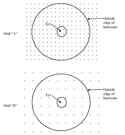
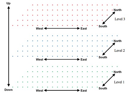
Aside from errors in the model initial condition, forecast errors in dynamical models can also arise because the physical equations they use cannot be solved exactly. The approximations that are made to solve the equations can introduce forecast error. What kinds of approximations are required depend partially on the model resolution. Model resolution refers to what size features can be explicitly represented in the model. Any features that are too small to be explicitly represented using the model’s mathematical equations must be parameterized, and approximations in the parameterization schemes can introduce forecast error. Some physical processes, even potentially important ones, are either too small scale or poorly understood, and are not included in dynamical models.

The easiest way to describe model resolution is to consider the subset of dynamical models that calculate the atmospheric variables at points on a grid (see diagram to the right). Let’s say we have one dynamical model that calculates the atmospheric variables on Grid “A” and another dynamical model that calculates the atmospheric variables on Grid “B”.

On Grid “A”, to the right, there are four grid points (where the atmospheric variables are calculated) inside the hurricane eye and twelve grid points surrounding the eye, while on Grid “B”, there are zero grid points inside the eye and only four grid points surrounding the eye. Since Grid “A” has more information in and around the eye than Grid “B” does, Grid “A” is able to give a better representation of the eye than Grid “B” can. Therefore, Grid “A” is said to have smaller grid spacing and higher resolution than Grid “B” does. Note that the grids shown above only represent one horizontal slice of the atmosphere, but grid-based dynamical models calculate the atmospheric variables on a vertical stack of grids so that the atmosphere is fully three-dimensional (from the surface to the higher levels of the atmosphere).

Schematic showing a vertical stack of grids, which could represent the three-dimensional atmosphere (or ocean). There are three levels with grid points in the top [level 3], middle [level 2], and bottom [level 1] grids shown with red, blue, and green dots, respectively).

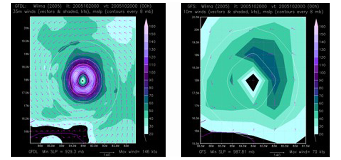
In theory, the higher the model resolution is, the better the model forecast will be, but in reality, many other complicating factors prevent this statement from always holding true, including errors introduced by the parameterization schemes. Also, increasing the model resolution requires much more computer resources, so a model with very high resolution may be too slow to be useful to hurricane forecasters.

Dynamical models that calculate the atmospheric variables over the entire earth are called global models. These global models are used not only to forecast the track and intensity of hurricanes, but also the general circulation of the entire atmosphere, including other weather systems like extratropical cyclones that are typically found in the mid-latitudes. Currently, the resolution of global models is sufficient to produce accurate hurricane track forecasts but is too low to produce accurate hurricane intensity forecasts. As supercomputer speeds increase, however, global models soon may be able to produce accurate intensity forecasts as well as track forecasts. One example of a global dynamical model is the U. S. National Weather Service Global Forecast System (GFS). Like other dynamical models, the GFS has a data assimilation scheme that reads in and utilizes measured atmospheric variables from many different observational platforms, including weather balloons, aircraft, satellites, radars, land-based weather instruments, ships, and buoys.

Even so, many more observations exist than are currently being assimilated into dynamical models. Thus, improved data assimilation techniques as well as increased model resolution and improved physics are needed to make full use of all available observations. In addition to the GFS, forecasters at the U.S. National Hurricane Center (NHC) often use the following global dynamical models:

• Canadian Meteorological Centre (CMC) Global Environmental Multiscale (GEM) Model
• European Center for Medium-range Weather Forecast (ECMWF) Model
• Navy Operational Global Atmospheric Prediction System (NOGAPS)
• United Kingdom Meteorological Office (UKMET) Model

Dynamical models that calculate the atmospheric variables in a limited area surrounding a hurricane are called regional models. On the boundary of the area covered by a regional model, atmospheric variables from a global model are passed across the boundary during the regional model forecast. This passing of atmospheric variables from the global model to the regional model is called the horizontal boundary condition. The main advantage of a regional model is that because it covers a smaller area than a global model, it can have higher resolution without requiring excessive computer resources, so it can make more accurate track and intensity forecasts.

Hurricane forecast model images showing a horizontal map of the wind speed (color shaded in knots- green colors indicate lighter winds, purple colors indicate stronger winds), wind direction (arrows), and atmospheric pressure (white contours) close to the sea surface in Hurricane Wilma (2005). The GFDL hurricane model (see paragraph to follow), shown in the left image, has higher resolution than the GFS model, shown in the right image. Therefore, the GFDL hurricane model is able to capture the small eye and the very high wind speeds in Wilma’s eyewall, but the GFS model cannot. Image credit: Timothy Marchok, NOAA/GFDL.

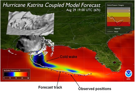
Three examples of regional models are NOAA’s Geophysical Fluid Dynamics Laboratory (GFDL) model , it’s U.S. Navy counterpart (GFDN), and NOAA’s Hurricane Weather and Research Forecasting (HWRF) model. All three of these models are coupled to a dynamical ocean model called the Princeton Ocean Model (POM). Coupling, or linking, a dynamical hurricane model to a dynamical ocean model allows the hurricane model to account for the interaction between a hurricane and the ocean. Also, these models use targeted observations from aircraft that fly inside the hurricane to create a very detailed and accurate initial condition of the hurricane in the model; having an accurate initial condition of the hurricane is critical for creating an accurate forecast. Finally, it should be noted that other countries have developed regional models for forecasting tropical cyclones in many areas around the world

GFDL coupled atmosphere-ocean model forecast of Hurricane Katrina (2005). At the start of the forecast, Katrina is located in the eastern Gulf of Mexico to the west of the southern tip of Florida. The model forecast track, indicated by the white line, is similar to actual observed track, indicated by the purple dots. As Katrina moves through the Gulf of Mexico towards Louisiana and Mississippi, it cools the sea surface temperature (SST), generating a cold wake, but the cold wake is not as cold where Katrina passes over the Loop Current (see Interaction between a Hurricane and the Ocean). The three-dimensional structure of the hurricane eye and eyewall a few hours before landfall are shown by the white “cloudy” areas. Katrina’s intensity (indicated here by central pressure and storm category, both from the GFDL model forecast [white line] and from the actual observed intensity [black line]) is shown in the graph in the upper-right part of the image. Image credit: NOAA/GFDL.

References

Additional Links on HSS